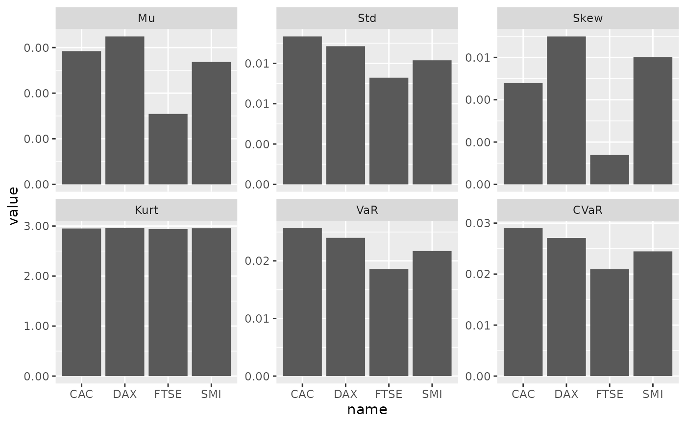
Summary Statistics for Empirical Distributions

Computes the mean, standard deviation, skewness, kurtosis, Value-at-Risk (VaR) and Conditional Value-at-Risk CVaR) under flexible probabilities.

empirical_stats(x, p = NULL, level = 0.01)

Arguments

x	A time series defining the scenario-probability distribution.
p	A probability vector. If NULL (the default) the standard 1 over N is used.
level	A number with the desired probability level. The default is level = 0.01.

Value

A tibble with 2 columns and 6 rows.

Examples

library(ggplot2)

x <- diff(log(EuStockMarkets))

calm_market  <- panic_copula(x = x, n = 1000, panic_prob = 0.00, dist = "normal")
panic_market <- panic_copula(x = x, n = 1000, panic_prob = 0.20, dist = "normal")

# Plot Calm market stats
emp_calm <- empirical_stats(calm_market$simulation, p = calm_market$p)
ggplot(emp_calm, aes(x = name, y = value)) +
 geom_col() +
 facet_wrap(~stat, scales = "free_y") +
 scale_y_continuous(labels = scales::number_format(accuracy = 0.01))


# Plot Panic market stats
emp_panic <- empirical_stats(panic_market$simulation, p = panic_market$p)
ggplot(emp_panic, aes(x = name, y = value)) +
 geom_col() +
 facet_wrap(~stat, scales = "free_y") +
 scale_y_continuous(labels = scales::number_format(accuracy = 0.01))