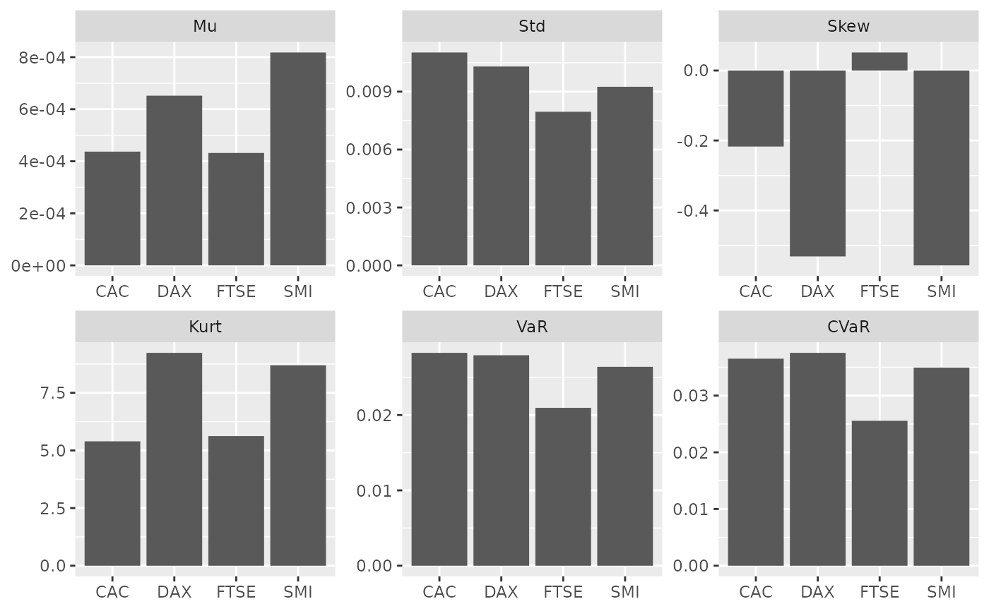
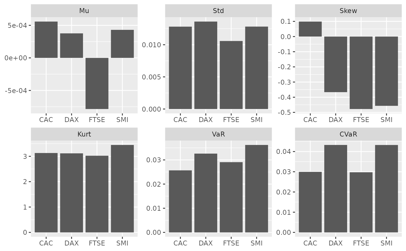
Computes the mean, standard deviation, skewness, kurtosis, Value-at-Risk (VaR) and Conditional Value-at-Risk CVaR) under flexible probabilities.
Usage
empirical_stats(x, p, level = 0.01)

# S3 method for default
empirical_stats(x, p, level = 0.01)

# S3 method for numeric
empirical_stats(x, p, level = 0.01)

# S3 method for matrix
empirical_stats(x, p, level = 0.01)

# S3 method for xts
empirical_stats(x, p, level = 0.01)

# S3 method for ts
empirical_stats(x, p, level = 0.01)

# S3 method for data.frame
empirical_stats(x, p, level = 0.01)

# S3 method for tbl_df
empirical_stats(x, p, level = 0.01)
Arguments
- x
A time series defining the scenario-probability distribution.
- p
An object of the
ffpclass.- level
A number with the desired probability level. The default is
level = 0.01.
Value
A tidy tibble with 3 columns:
stat: a column with
Mu,Std,Skew,Kurt,VaRandCVaR.name: the asset names.
value: the computed value for each statistic.
Examples
library(dplyr, warn.conflicts = FALSE)
library(ggplot2)

ret <- diff(log(EuStockMarkets))

# with equal weights (standard scenario)
ew  <- rep(1 / nrow(ret), nrow(ret))
empirical_stats(x = ret, p = as_ffp(ew)) %>%
  ggplot(aes(x = name, y = value)) +
  geom_col() +
  facet_wrap(~stat, scales = "free") +
  labs(x = NULL, y = NULL)


# with ffp
exp_smooth <- exp_decay(ret, 0.015)
empirical_stats(ret, exp_smooth) %>%
  ggplot(aes(x = name, y = value)) +
  geom_col() +
  facet_wrap(~stat, scales = "free") +
  labs(x = NULL, y = NULL)
